Examining Memory and Timing

In this example we show how to load the core diagnostic files (core.memory.csv, core.timing.csv, and core_diag.json) that POLARIS writes when run with --dump_core_diagnostics N (and, for the timing file, also --dump_core_diagnostics_timing).

See the memory/runtime section of the POLARIS system architecture documentation for more details.

from pathlib import Path
import json
import re

import matplotlib.cm as cm
import matplotlib.colors as mcolors
import matplotlib.pyplot as plt
import pandas as pd
import seaborn as sns

from polaris.utils.file_utils import get_caller_directory


def clean_manager_name(df):
    df["manager"] = df["manager"].str.replace(re.compile("<.*>"), "", regex=True)
    df["manager"] = df["manager"].str.split("::").str[-1]
    df["manager"] = df["manager"].str.replace("_Implementation", "")
    return df


output_dir = get_caller_directory() / "data"

# Load core_diag.json — contains whole-run thread and sub-iteration timing.
# | field | meaning |
# | --- | --- |
# | `num_threads` | number of worker threads |
# | `revision_count` | total simulation steps (revisions) processed |
# | `threads[i].step_ms` | time thread i spent doing work |
# | `threads[i].wait_ms` | time thread i spent idle at gates |
# | `threads[i].wait_pct` | idle fraction for thread i |
# | `total_step_ms` / `total_wait_ms` | sums across all threads |
# | `sub_iterations[k].step_ms` | summed thread work time for sub-iteration k |
# | `sub_iterations[k].wait_ms` | summed thread wait time for sub-iteration k |
# | `sub_iterations[k].utilisation_pct` | step / (step + wait) × 100 |
core_diag_path = output_dir / "core_diag.json"
if core_diag_path.exists():
    with open(core_diag_path) as f:
        core_diag = json.load(f)
    num_threads = core_diag["num_threads"]
    print(f"core_diag.json: {core_diag['revision_count']} revisions, {num_threads} threads")
else:
    core_diag = None
    num_threads = 10
    print("core_diag.json not found — running without it")

core_diag.json: 711540 revisions, 10 threads

## General timing

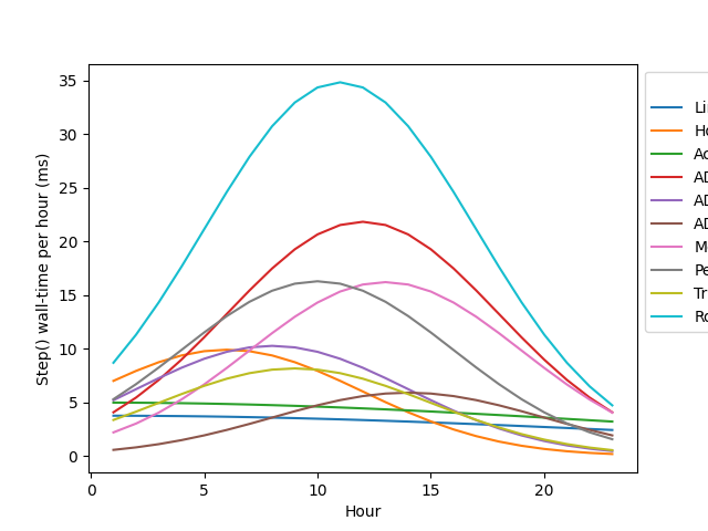
core.timing.csv records cumulative wall-time spent in each component manager’s Step() plus how many times Step() was called. Schema:

column | meaning |

— | — |

iteration | simulation iteration |

manager, component_id | as for memory |

step_call_count_cumulative | total Step() invocations since simulation start |

step_time_ns_cumulative | total ns inside Step() since simulation start |

Because both counters are cumulative, diff between consecutive rows to get per-window values.

timing = clean_manager_name(pd.read_csv(output_dir / "core.timing.csv"))
timing = timing.drop_duplicates(subset=["iteration", "manager"], keep="first")
timing["Hour"] = timing["iteration"] / 3600

timing = timing.sort_values(["manager", "iteration"])
timing["calls_in_window"] = (
    timing.groupby("manager")["step_call_count_cumulative"].diff().fillna(timing["step_call_count_cumulative"])
)
timing["time_ms_in_window"] = (
    timing.groupby("manager")["step_time_ns_cumulative"].diff().fillna(timing["step_time_ns_cumulative"]) / 1_000_000
)

Per-manager Step() time per hour, top 10 by total wall-time.

total_time_per_manager = timing.groupby("manager")["time_ms_in_window"].sum()
slowest = total_time_per_manager.sort_values(ascending=False).head(10).index
plot_df = timing[timing["manager"].isin(slowest)].sort_values("iteration")
plot_df = plot_df[plot_df["Hour"] > 0.5]

ax = sns.lineplot(plot_df, x="Hour", y="time_ms_in_window", hue="manager")
ax.set_ylabel("Step() wall-time per hour (ms)")
sns.move_legend(ax, "upper left", bbox_to_anchor=(1, 1))

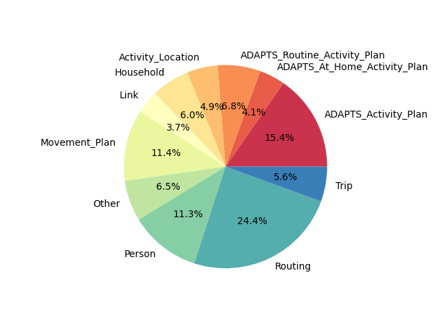
Top 10 managers by total Step() time — pie chart.

final_row = timing[timing["Hour"] > 0.5].groupby("manager").sum()[["time_ms_in_window"]].reset_index()
final_row = final_row.sort_values("time_ms_in_window", ascending=False).reset_index(drop=True)

top_n = 10
final_row["category"] = final_row["manager"].where(final_row.index < top_n, "Other")
pie_data = final_row.groupby("category")["time_ms_in_window"].sum().reset_index()
colors = sns.color_palette("Spectral", len(pie_data))
ax = pie_data.plot.pie(
    autopct="%1.1f%%", ylabel="", y="time_ms_in_window", legend=False, colors=colors, labels=pie_data["category"]
)

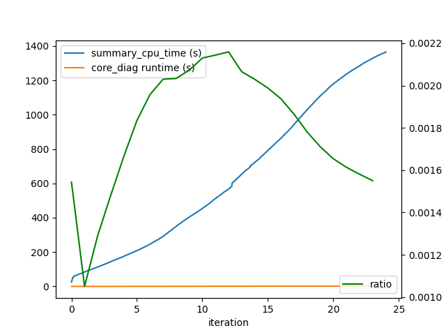
This doesn’t tell the whole story however, as there is also the matter of threading efficiecy that needs to be accounted for. For example, the intersection compute step flow manager is the slowest by cpu-clock time, but it is also the most efficiently threaded, so the actual wall clock time spent in this manager is actually much higher than the wall-clock time would suggest. The overall efficiency can be measrued by comparing the cpu time from the core-diagnostic CSV to the wall clock time from the summary CSV. The ratio of these can give us an estimate of efficiency (shown in green)

summary = pd.read_csv(output_dir / "summary.csv", index_col=False)
wall_time = summary["wallclock_time(ms)"].iloc[-1]
summary["summary_cpu_time (s)"] = summary["wallclock_time(ms)"] * num_threads / 1000
summary["simulated_hour"] = summary["simulated_time"] / 3600
summary.plot(x="simulated_hour", y="summary_cpu_time (s)")
ax = plt.gca()
tmp = timing.groupby("iteration")["step_time_ns_cumulative"].sum().reset_index()
tmp["core_diag runtime (s)"] = tmp["step_time_ns_cumulative"] / 1_000_000 / 1000
tmp["iteration"] = tmp["iteration"] / 3600
tmp.plot(ax=ax, x="iteration", y="core_diag runtime (s)")

summary_for_join = summary.set_index("simulated_hour")
tmp = tmp.set_index("iteration").join(summary_for_join, how="left")
tmp["ratio"] = tmp["core_diag runtime (s)"] / tmp["summary_cpu_time (s)"]
ax2 = ax.twinx()
sns.lineplot(x=tmp.index, y=tmp["ratio"], ax=ax2, label="ratio", color="green")
ax2.set_ylabel("Ratio")
ax2.legend(loc="lower right")

<matplotlib.legend.Legend object at 0x7dea04d649b0>

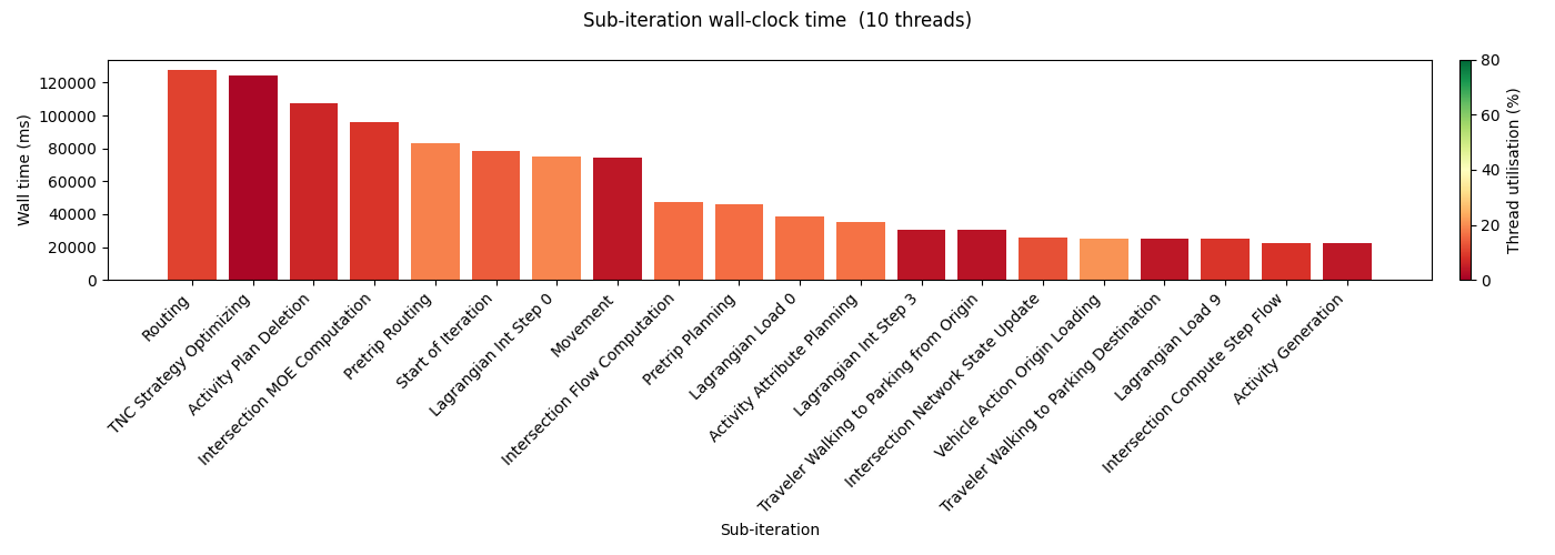
## Sub-iteration timing

Because of the way threading is setup, it’s hard to attach threading efficiency directlyy to each manager, as each thread may be working on a different manager at any given time. However, we can break things down by sub-iteration and (in practice) generally there will only be a single manager running per sub-iteration.

Sub-iteration timing comes from core_diag.json (requires core diagnostic timing enabled). Each sub-iteration corresponds to a specific class of agent/manager work. A utilisation near 100 % means all threads were busy for the full wall-clock window; a low value indicates load imbalance — threads finishing early and sitting idle.

common_sub_iter_names = {
    0: "Start of Iteration",
    2: "Events Update",
    3: "Routing",
    9: "Link Supply Update",
    10: "Intersection Compute Step Flow",
    12: "Intersection Flow Computation",
    13: "Lagrangian Int Step 0",
    14: "Lagrangian Load 0",
    15: "Pretrip Planning",
    16: "Pretrip Routing",
    17: "Activity Attribute Planning",
    18: "Movement",
    22: "Lagrangian Int Step 3",
    28: "Activity Generation",
    30: "Lagrangian 5",
    40: "Traveler Walking to Parking Destination",
    41: "Traveler Walking to Parking from Origin",
    42: "Lagrangian Load 9",
    44: "Vehicle Action Transfer",
    46: "Vehicle Action Origin Loading",
    51: "Intersection Network State Update",
    53: "Intersection MOE Computation",
    58: "Demand Output Writing",
    700: "TNC Strategy Optimizing",
    9823247: "Activity Plan Deletion",
}

if core_diag is not None and "sub_iterations" in core_diag:
    sub_df = (
        pd.DataFrame(
            [
                {
                    "sub_iteration": common_sub_iter_names.get(int(k), k),
                    "step_ms": v["step_ms"],
                    "wait_ms": v["wait_ms"],
                    "wall_ms": v["wait_ms"] + v["step_ms"],
                    "utilisation_pct": v["utilisation_pct"],
                }
                for k, v in core_diag["sub_iterations"].items()
            ]
        )
        .sort_values("sub_iteration")
        .reset_index(drop=True)
    )

    sub_df = sub_df.sort_values("wall_ms", ascending=False).head(20)

    cmap = cm.RdYlGn
    norm = mcolors.Normalize(vmin=0, vmax=80)
    bar_colors = [cmap(norm(u)) for u in sub_df["utilisation_pct"]]

    fig, ax = plt.subplots(1, 1, figsize=(14, 5))
    ax.bar(range(len(sub_df)), sub_df["wall_ms"], color=bar_colors)

    ax.set_xticks(range(len(sub_df)))
    ax.set_xticklabels(sub_df["sub_iteration"], rotation=45, ha="right")
    ax.set_xlabel("Sub-iteration")
    ax.set_ylabel("Wall time (ms)")
    fig.suptitle(f"Sub-iteration wall-clock time  ({num_threads} threads)")

    sm = cm.ScalarMappable(cmap=cmap, norm=norm)
    sm.set_array([])
    cbar = fig.colorbar(sm, ax=ax, orientation="vertical", fraction=0.03, pad=0.02)
    cbar.set_label("Thread utilisation (%)")
    cbar.set_ticks([0, 20, 40, 60, 80])

    plt.tight_layout()
    plt.show()
    sub_df
else:
    print("core_diag.json not found or does not contain sub_iterations")

## Memory usage

core.memory.csv records one row per (iteration × component manager × block) every –dump_core_diagnostics N iterations. The schema is:

column | meaning |

— | — |

iteration | simulation iteration (seconds since 00:00) |

manager | component manager name |

component_id | numeric id |

num_active_blocks | total blocks currently active for this manager |

cell_size | per-cell size in bytes |

block_memory_managed_by | worker thread that owns this block |

block_num_allocated | live objects in this block |

block_num_cells | total cells in this block |

block_excess_bytes | wasted capacity (= (num_cells - num_allocated) * cell_size) |

mem = clean_manager_name(pd.read_csv(output_dir / "core.memory.csv"))

mem["bytes_used"] = mem["block_num_allocated"] * mem["cell_size"]
per_manager = mem.groupby(["iteration", "manager"], as_index=False)["bytes_used"].sum()
per_manager["Hour"] = per_manager["iteration"] / 3600
per_manager["MBytes"] = per_manager["bytes_used"] / (1024 * 1024)

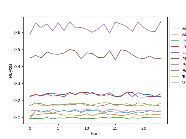
Plot the 10 component managers with the highest peak memory use.

n = 10
peak_mem = per_manager.groupby("manager")["MBytes"].max()
biggest_mem_usage = peak_mem.sort_values(ascending=False)[0:n].index
plot_df = per_manager[per_manager["manager"].isin(biggest_mem_usage)]

ax = sns.lineplot(plot_df, x="Hour", y="MBytes", hue="manager")
sns.move_legend(ax, "upper left", bbox_to_anchor=(1, 1))

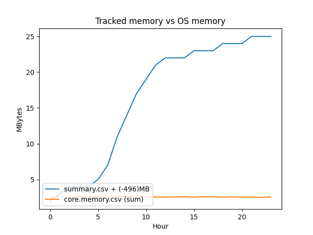
Tracked object memory vs OS-reported physical memory. The delta reflects dynamically allocated memory inside objects (vectors, maps, etc.) that POLARIS doesn’t track. On Grid we typically see a 300+ MB delta that drifts upward even when the tracked total goes down (memory isn’t reliably released back to the OS).

total_per_hour = per_manager.groupby(per_manager["Hour"].astype(int))["MBytes"].sum()

summary_mem = pd.read_csv(output_dir / "summary.csv")
cols = list(summary_mem.columns) + ["unknown"]
summary_mem = summary_mem.reset_index()
summary_mem.columns = cols
summary_mem["hour"] = (summary_mem.simulated_time / 3600).astype(int)
summary_mem = summary_mem.groupby("hour")[["physical_memory_usage"]].max()

offset = round(summary_mem.physical_memory_usage.iloc[0] - total_per_hour.iloc[0])
summary_mem["physical_memory_usage"] = summary_mem.physical_memory_usage - offset

ax = sns.lineplot(summary_mem, x="hour", y="physical_memory_usage", label=f"summary.csv + (-{offset})MB")
sns.lineplot(x=total_per_hour.index, y=total_per_hour.values, ax=ax, label="core.memory.csv (sum)")
ax.set_xlabel("Hour")
ax.set_ylabel("MBytes")
ax.set_title("Tracked memory vs OS memory")
sns.move_legend(ax, "lower left")