Population Synthesis Analysis

After a population has been synthesized and used in a POLARIS run, you typically want to verify that the synthetic population actually matches the control marginals it was built from. The PopsynComparator class does this comparison and produces validation plots.

For working with the synthetic population itself (loading, modifying, saving), see the Population page.

Quick start

If your model is in a standard US Census-based context, the easiest way to get started is PopsynComparator.from_dir:

from polaris.analyze.popsyn_analysis import PopsynComparator
from polaris.prepare.popsyn.linker_file import LinkerFile

linker = LinkerFile(my_run_dir / "linker_file.txt", project_dir=my_run_dir)
comparator = PopsynComparator.from_dir(my_run_dir, sample_factor=1.0, linker_file=linker)

comparator.summarise()                              # logs aggregate match rates
comparator.generate_comparison_plots(geo_level=0, linker=linker)  # scatter plots

from_dir loads the population from the demand database (using the same fast HDF5 cache as Population.from_dir) and constructs a default USCensusMapping strategy automatically.

Geographic mapping strategies

Validation has to bridge three geographic levels:

1. household location — whatever lives in the household.location column of the demand database. This is model-specific.

2. popsyn region — the geographic unit at which control marginals are defined (e.g., a US Census tract).

3. survey region — the geographic unit at which the seed sample is provided (e.g., a US PUMA).

The GeoMappingStrategy interface abstracts over this. Two implementations ship with polaris-studio:

USCensusMapping

Maps household.location to a US 2010 Census tract and then to a PUMA using the standard Census Bureau crosswalk. It supports three encodings for the location column, selected via LocationMode:

Mode	household.location content	Extra data needed
POI	small POI IDs that index supply_db.location	supply_db (auto-loaded)
TRACT	full 10-11 digit Census tract GEOIDs	none
BLOCK	15 digit Census block GEOIDs	block_to_puma DataFrame

The recommended constructor is from_location_mode, which loads all required crosswalks up front (so any I/O errors surface immediately rather than at plot time):

from polaris.analyze.geo_mapping import USCensusMapping, LocationMode

geo_mapping = USCensusMapping.from_location_mode(
    location_mode=LocationMode.POI,
    supply_db=my_run_dir / "MyModel-Supply.sqlite",
    puma_id_contains_state_id=False,
)

If location_mode is None, it defaults to POI when supply_db is available and otherwise TRACT.

Avoiding the remote crosswalk download. By default the PUMA-to-tract crosswalk is downloaded from the Census Bureau on first use. To use a local copy (for testing, offline work, or pinning a specific vintage), pass puma_to_tract_csv:

geo_mapping = USCensusMapping.from_location_mode(
    location_mode=LocationMode.TRACT,
    puma_to_tract_csv=my_data_dir / "2010_Census_Tract_to_2010_PUMA.txt",
)

The CSV must follow the standard Census Bureau format with STATEFP, COUNTYFP, TRACTCE, and PUMA5CE columns.

CustomMapping

For non-US regions or any model whose geography doesn’t fit the Census tract→PUMA hierarchy, supply your own mapping DataFrames:

from polaris.analyze.geo_mapping import CustomMapping

geo_mapping = CustomMapping(
    popsyn_region_col="sa1_zone",
    survey_region_col="sa3_zone",
    location_to_popsyn=location_to_sa1_df,  # columns: ["location", "sa1_zone"]
    popsyn_to_survey=sa1_to_sa3_df,         # columns: ["sa1_zone", "sa3_zone"]
)

comparator = PopsynComparator(population, 1.0, linker, geo_mapping=geo_mapping)

The two DataFrames must be complete: any household with no match in location_to_popsyn or any popsyn region with no match in popsyn_to_survey will raise.

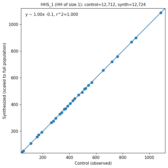
Producing validation plots

generate_comparison_plots produces a grid of scatter plots — one per control variable (household size, age band, race, etc.) — comparing the control marginal on the x-axis against the synthesized count on the y-axis. The geo_level argument controls aggregation: 0 for popsyn region (tract), 1 for survey region (PUMA).

Each subplot shows the per-region observed vs. synthesized counts, an OLS regression line with r², and a y=x reference (dotted grey). A good fit hugs the y=x line:

For a single comparison, use the lower-level PopsynComparator.compare_synthpop_to_controls directly — it returns the underlying merged DataFrame so you can inspect or further analyze the data:

comp = PopsynComparator.compare_synthpop_to_controls(
    control_data, synth_data,
    sample_fac=1.0,
    geo_col_index=0,
    compare_name="HHS_1",
    ax=my_axes,
)
# comp has columns ["control", "synthesized"], one row per geo unit

The plotting helper plot_scatter(obs, synth, ...) is also exposed as a class method if you want to draw the same y=x reference + OLS overlay on your own data.

API Reference

polaris.analyze.popsyn_analysis.PopsynComparator
polaris.analyze.geo_mapping.GeoMappingStrategy	Strategy for mapping households to popsyn and survey regions.
polaris.analyze.geo_mapping.USCensusMapping	US Census-based geographic mapping (tract → PUMA).
polaris.analyze.geo_mapping.CustomMapping	Custom geographic mapping via user-provided DataFrames.
polaris.analyze.geo_mapping.LocationMode	How household home locations are encoded in the demand database household.location column.