Random Choice

Random choice is at the heart of all simulation modelling and POLARIS is no different. There are many common pitfalls that new practitioners will encounter as they start using computational random number generation to simulate decision making processes. Where we can we’ve tried to round off some of the rough edges and encapsulate good practices into the random number classes in RNG_Components.

In practice, the vast majority of random numbers in POLARIS follow either a uniform or normal distribution and we provide two classes that wrap these:

1. UniformRNG

2. NormalRNG

They make use of std library implementations for the distributions as well as the RNG (this is chosen to be a linear congruential engine rather than a Mersene Twister as they are significantly faster to instantiate and satisfy all required statistical properties). To enable reproducible draws, both classes expose RNG seeding (seed) and access to the underlying generator (get_rng) for use in alternate distributions. This is discussed further below.

To illustrate the intended usage of these classes, let us consider a simple uniform random number generator:

RNG_Components::Implementations::UniformRNG rng(1, 1);

The easiest type of random choice to make is a simple binary one. For example: “does this agent have a bus-pass?”

double bus_pass_holding_rate = 0.45;
bool has_bus_pass = rng.evaluate_probability(bus_pass_holding_rate); // returns true 45% of the time

The second most common type of decision is to choose an element from a set of things.

vector<tMT::zone_type*>& zones = get_zones(); // get some zones to choose from
tMT::zone_type* chosen_zone = rng.choose_element(zones);  // Choose a zone uniformly

This is a very common operation and has been implemented to be as fast as possible - as we are assuming a uniform probability of all elements, we can calculate the index of the chosen element using constant time index algebra.

However, it’s often required to move away from uniform choice and add some weighting function. For example we may want to choose our zone with a probability based on its population.

In that case we can use two versions of choose_element that take either a weighting function or a standard library discrete_distribution.

// define a weight function that is just the population of the zone
auto get_population = [=](tMT::zone_type* z) { return z->num_people(); };

// choose a zone using that weight function
tMT::zone_type* chosen_zone = rng.choose_element(zones, get_population);

We provide two ways to generate the appropriate discrete_distribution object from either our zones and weight function or from pre-existing weights.

// Pre-compute a std::distribution based on the things and a weight function
discrete_distribution<> weight_dist = preprocess_distribution(zones, get_population);

// Or if we already have a set of weights from somewhere else
discrete_distribution<> weight_dist = preprocess_distribution(weights);

// Make choice
tMT::zone_type* chosen_zone = rng.choose_element(zones, weight_dist);

These two forms have slightly different performance characteristics and which to use will be based on the type of choices being made and the cost/complexity of the weight function. The general rule is that if your weight function is simple enough and you are only drawing a small number (i.e. less than 3) of times, you should use the form which takes a weight function. If you have a complex weight function or are making repeated selections you should take the time to pre-compute the discrete_distribution.

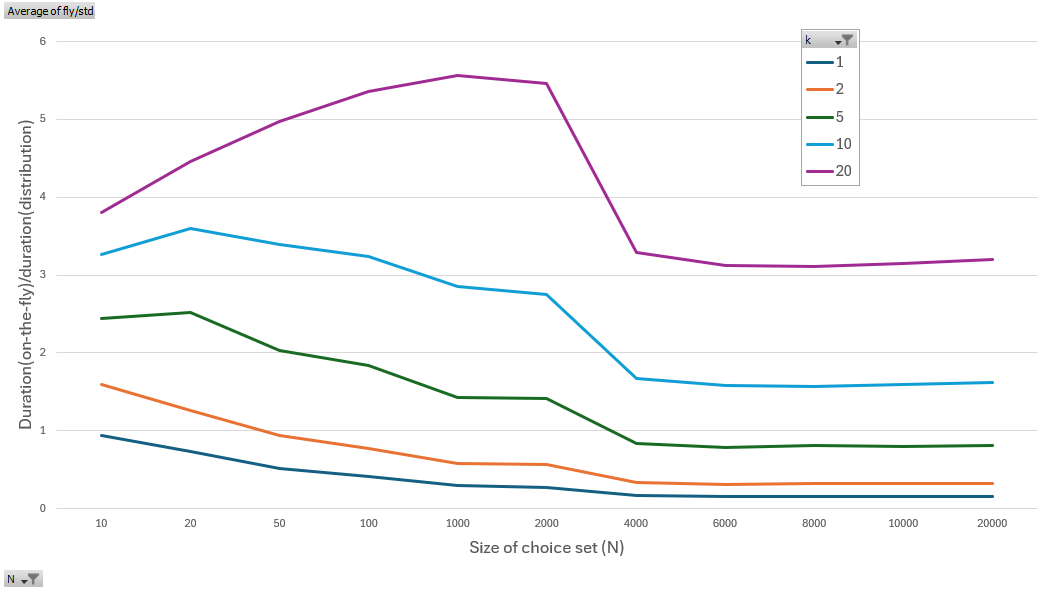
This can be seen in the following charts which show the relative time taken for varying number of draws (k) from a vector of random weights with varying size (n). Values less than 1.0 indicate that the ‘on-the-fly’ version is faster, while >1.0 means that precomputing is faster by the given value (i.e. 2.0 = precomputing takes half the time of ‘on-the-fly’).

This was calculated using a weight function which was marginally complex w=rand()^4+10000. This is representative of the number of clock cycles required to call a simple getter function on a c++ object.

Important

When using more complex weight functions w=pow(rand(), 1.7) the pre-computed version was always faster.

Simulation variance and reproducability

TODO - flesh this out with guidelines on

• “run things many times with different seeds”, on

• using different rngs for different parts of the program (e.g. each person),

• reproducability (seed each person with person_id so same order of daily decisions are exactly the same),

• current sources of noise (assignment - cars entering link are in random order so travel times vary),

• variation reduction re person decisions (MXL models, planned), etc