Lagrangian Coordinates Model#
The mesoscopic model is derived from macroscopic models (LTM, Newell’s model) which is an approximation of traffic flow as fluids containing three key variables, density, flow and speed. Most of those models are derived from what is called the Eulerian coordinates by which those variables are mapped into space and time. This is clear on the famous cell transmission model in which quantities (primarily density) is computed for every cell (space) at all times. Nevertheless, it is possible to use other coordinates to such as the Lagrangian Coordinates. The Lagrangian Coordinates follow an unit of the fluid (a particle) over time. Therefore, instead of discretizing the space into cells of size \Delta x, the Lagrangian coordinates split the fluid into particles of size \Delta n. For traffic flow this has an intuitive interpretation as it is vehicles coordinates similar to a microscopic models. However, but it is important to present the key distinctions to microscopic models: - In Lagrangian coordinates the particle (vehicles) has a size \Delta n that can take any value. In microscopic model each vehicle is one (equivalent to \Delta n=1). - Lagrangian coordiantes does not have multiple lanes (at least in this implementation) on the same stream, therefore if a vehicle has multiple lanes vehicles would be able to follow more closely. For instance, if vehicles in one lane travels at free-flow speeds for spacing around 50m in Lagrangian Coordinates if the link has 5 lanes, vehicles could keep free-flow speed at spacing of 10m. In other words, the effective spacing is the spacing with respect to the leading vehicle multiplied by the number of lanes. - As it is a “single pipe”, there is no lane changing in this model.
On the other hand, one aspect that the Lagrangian Coordinates inherit from microscopic model is the easiness to extend the models with the new features, particularly for capturing heterogeneous vehicles. We present here the modeling assuming homogeneous vehicles, but later we discuss some features that take advantage of this aspect.
Baseline model#
The model assumptions is equivalent to the mesoscopic model – a LWR model with a triangular fundamental diagram. The link description and parameters are described in the Figure below. The link has a length and a pocket length; the through pocket has always the number of lanes of the link and additionally it may contain left and right pockets.
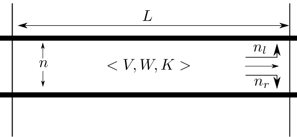
Traffic parameters are determined by the triangular fundamental diagram parameters: $v_f$ is the free-flow speed, $\omega$ for shock-wave speed and $k_j$ is the per-lane jam density. The jam spacing, $s_j$, is the inverse of the jam spacing ($s_j=\frac{1}{k_j}$). Note that we could describe the model in terms of reaction time and jam spacing, but we use the same notation and parameters as the previous modeling \cite{de2019mesoscopic} in Eulerian coordinates. At all times, the spacing $s$ which the particle $j$ experiences depends on its position, $X(j,i)$ and the position of its leader $X(j-1, i)$:
and the speed of any particle depends on the spacing $s$ in which for a triangular fundamental diagram becomes:
Vehicle speeds are updated based on spacing s(j,i) and position update as:
Therefore, based on the state of each vehicle, new speeds and updated positions can be computed in each link for every vehicle.
Observe in the equations above that it is assumed there is always a leading vehicle and the spacing can be computed. There are two important elements on this aspect. First, the leading vehicle might be in one of the pockets that may have a different number of lanes if the vehicle is on the link portion. In this case, the spacing is scaled based on the ratio of number of lanes in the pocket and in the link to determine an equivalent spacing to be used. Second, the vehicle can be the “first” in the link and the leading vehicle might be in the downstream link. In this case, the spacing is assumed to be infinity; however, the node model takes care of this element to determine whether the vehicle is able or not to transfer to the next link. In so doing, the position of the vehicle might be revised to reflect the spacing of the new leader in the next link.
Node Models and Vehicle Transition#
Since the model is equivalent to the mesoscopic model (LWR model + triangular fundamental diagram), the node models in Lagrangian Coordinates model use similar modeling as the mesoscopic node models, but the demand and supplies are computed differently.
Demand and supply are computed as:
where $x^d(i)$ and $x^u(i)$ are the positions of the most downstream and upstream vehicle, respectively, and $S(x)$ is the step function (1 if $x \geq 0$ and 0 otherwise). The q^d and q^u are the capacity state variables and are computed in the same way as the mesoscopic model:
The capacity downstream may be specific to the pocket and its number of lanes as well.
The only distinction with respect to the mesoscopic model is that the maximum flow in a single time-step is 1 whereas in the mesoscopic model is always an integer number. Please refer to the mesoscopic node models for further details.
Multiclass Extension#
All the elements presented so far assumed that all vehicles were homogeneous this includes the free flow speed, v_f, the shock-wave speed, w, and the jam spacing, s_j. This also determines the link capacity and the update of the capacity state variables. One advantage of the Lagrangian Coordinates is the possibility to easily introduce vehicle-specific behaviors. This is implemented by changing the speed-spacing equation and ensuring consistency on the boundaries:
Speed equation: elements related to jam spacing, free-flow speed and shock-wave speed (related to reaction time) is specific to each vehicle. In the input parameters, speed and shock wave speed (reaction time) are specified as multipliers based on link type (expressway, arterial, local) and jam spacing (jam density) as a shift with respect to passenger vehicle specified in meters by mode. For instance, light duty truck 5m and 10m for heavy-duty trucks.
The capacity used to inform the capacity related state variables, $q^a$ and $q^d$ are computed based on the relevant vehicle (most upstream or downstream vehicle); same for free-flow speed and jam spacing in the demand and supply equations.
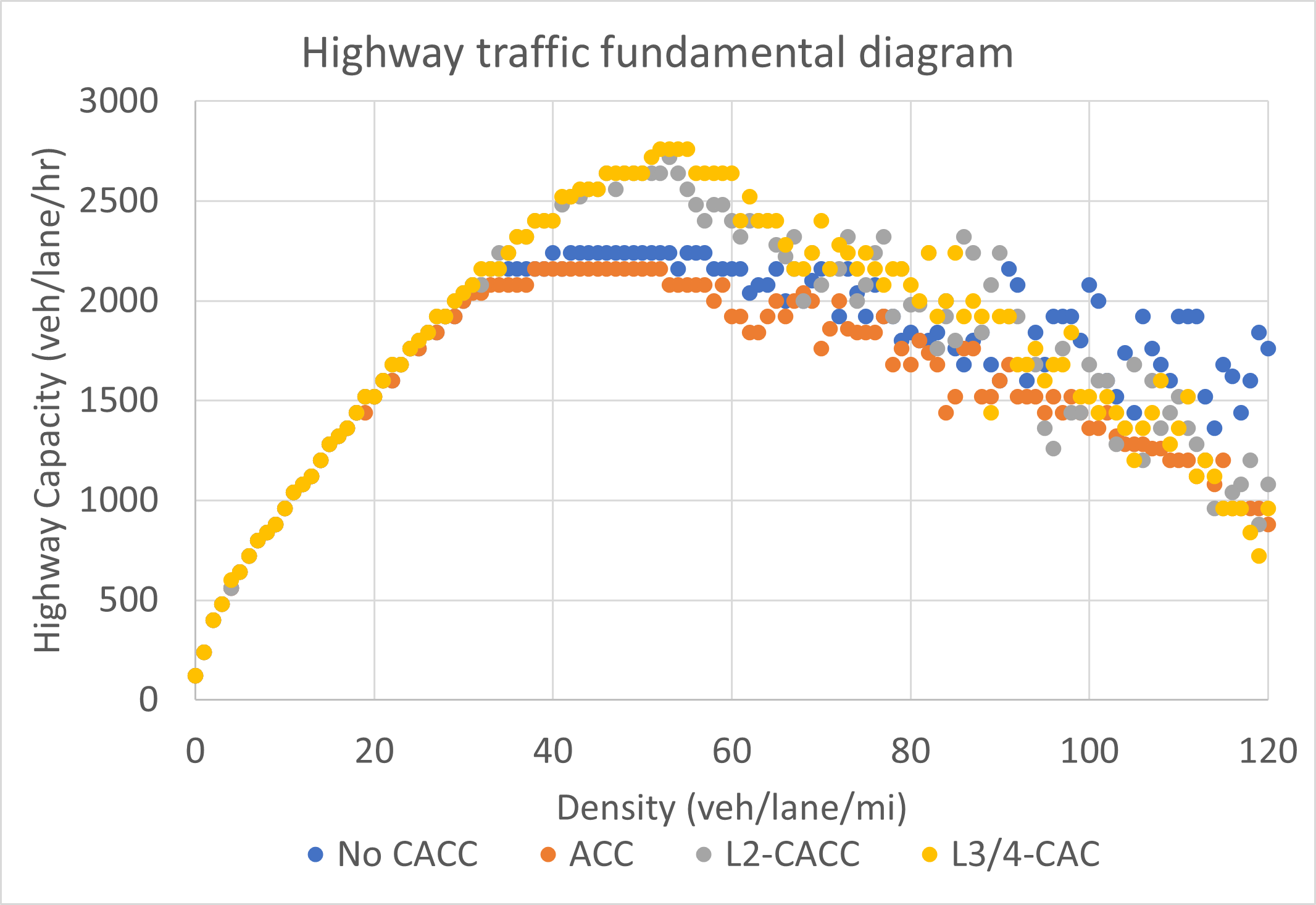
The Figure below shows a common setting, with trucks having lower free-flow speed and higher jam spacing, and automated vehicles with lower reaction time.
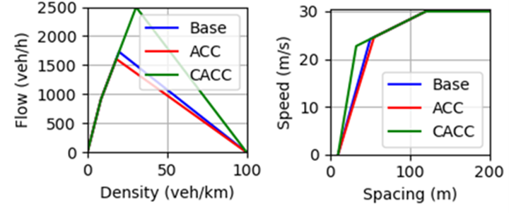
This is the resulting approximate flow-density relationship from the simulation results based on the settings above.
These runs were conducted with these settings:
"multiclass_definition": "LINK_TYPE_BY_REGULAR_AV_TRUCK",

"multiclass_av_reaction_multiplier_expressway": 0.6,

"multiclass_av_reaction_multiplier_local": 1.0,

"multiclass_av_reaction_multiplier_signalized": 1.0,

"multiclass_freight_reaction_multiplier_expressway": 1.0,

"multiclass_freight_reaction_multiplier_local": 1.0,

"multiclass_freight_reaction_multiplier_signalized": 1.0,
Key parameters that may interfere in the Lagrangian Coordinates:
"num_lagrangian_sub_steps": 10
num_lagrangian_sub_steps controls the time step. The effective time-step is simulation_interval_length_in_seconds/num_lagrangian_sub_steps. Most of the time this value can be set to 1. If required lower time steps, especially with traffic_scale_factor > 0.5, then use it to set effective time steps of 0.5s/0.25s, etc.
Multiclass Settings and Parameters#
“minimum_pocket_length”: this parameter controls how small might be a pocket. Generally, is advisable to be higher than the maximum distance a vehicle travel in one time step.
“use_piecewise_linear_fd”: this allows to use a fundamental diagram with two different steps in the uncongested branch of the fundamental diagram instead of the triangular fundamental diagram. This adds two other parameters:
"piecewise_linear_fd": true,

"beta_piecewise_linear_fd": 2.0,

"gamma_piecewise_linear_fd": 0.25
Beta > 1 is a multiplier of the critical density compared to the critical density of the triangular fundamental diagram for the same capacity and free-flow speed. Gamma specifies at which point the speeds differ from the free-flow speed (0.25 means that at 25% of critical density).