Traffic Flow Model#
POLARIS features a traffic simulation module that is key to capture emerging congestion based on the agents’ demand decisions such as destination and mode choices. With the routing, the traffic flow simulation returns travel times for “driven” modes (SOV, TNC, LD_TRUCK, etc.) in the perspective travelers (i.e., trip time from origin to destination) as well as from the network key performance indices (KPI’s) such as speed, delay, density, etc. in time and space.
There are specific aspects to the traffic simulation that are relevant for POLARIS scenarios, but its level of details, harmony with model capabilities, and calibration data may not always fit into the overall scenario. For instance, a coordinated adaptive signal control with vehicle-to-vehicle communication and such are interesting elements, but often the required level of details that is unsuitable to be applied in the large-scale scenarios. For those cases, there are two elements that can turn a study on a specific impact (such as the adaptive signal and vehicle-to-vehicle communication):
Micro-to-Meso indirect adaptation:
Behavioral change in a target area through Application Programming Interface:
Multi-scale modeling (work in progress)
These aspects will be briefly considered when discussing specifics of each modeling. In addition, the API documentation can be found here.
Brief Network Description#
Several of the elements discussed here are also part of the network documentation. Here, we discuss the traffic flow impacts and concepts. We refer to that documentation for specific details on how to input parameters and such.
Links#
POLARIS contains multiple link types (multimodal, walk, road, etc.) and here are limiting to the road links that are defined in the “Link” table on the supply database. In that table, links have an identifier and length and connects two nodes (node_a, node_b). Note that the existence of the links and nodes do not imply the existence of a directed link that starts in node_a and ends in node_b and the opposite. There is a link starting node_a (node_b) and ending in node_b (node_a) if lanes_ab (lanes_ba) is greater than zero. Internal to POLARIS, these links from lanes_ab and lanes_ba are the directed links with the following identifiers: 2link + 0 -> link from node_a to node_b (lanes_ab > 0) 2link + 1-> link from node_b to node_a (lanes_ba > 0) From now on, we are describing parameters and elements of unidirectional link. Just keep in mind that the imputation of these parameters might be in the Link table itself (lanes_ab, fspd_ab, lanes_ba, fspd_ba, etc.) or in associated tables, but here we discuss as unique parameters (lanes, fspd, etc.)

A schematic of the link is represented in the Figure. Each link has a length, number of lanes and may contain left or right pockets with some length (Table Pocket). The through pocket has the same characteristics (namely, lanes) as the link itself. Moreover, there can be a stop sign at the end of the link (Table Sign). Along with the number of lanes and length, the free-flow speed (fspd_ab/fspd_ba). They are applicable for the current supported models (Mesoscopic/Lagrangian), but the plan is to support further models either with less or higher level fidelity. Therefore, not all parameters have an impact in all models and some of the models have specific parameters that is not covered in this section.
Nodes#
Opposite from the links that contains multiple parameters and traffic flow parameters, nodes are just link endpoints as far as the traffic simulation goes with the exception of the traffic signal.
The single parameter for node is the control_type (Node table) that can be one of the following:
No control: no stop sign in any of the inbound links and no signal control defined. The typical case is freeway merges and diverges.
Two-way (not all) stop: some of not all the inbound links have a stop sign. Typical case is local roads accessing minor or major roads.
Four-way (all) stop: all inbound links have a stop sign. Typical case is local roads.
Signalized: there is a complete record in the Signal and nested tables.
Connection#
Every node has a set of inbound and outbound links; however, for a given inbound link it is not always possible to reach any outbound link. In fact, the most common case is that some outbound link is not accessible as some movements are prohibited. For instance, the most common case is to not allow u-turns. In POLARIS, a pair of unique inbound and outbound link defines a connection. Often in documentation or within the POLARIS structures, the name “movement” also appears. Unless otherwise stated, they are synonyms as far as traffic simulation documentation goes. Each connection contains some associated attributes that may have impact in the simulation result. Namely:
Num_turn_lanes: how many lanes are accessible for the particular connection. It defines the capacity of the turn in the mesoscopic model.
Type and Direction: type determines the movement vehicles perform (left, right, thru/through, u-turn) and direction determines the inbound link movement direction (eastbound, westbound, etc.). Based on these attributes, POLARIS determines whether two connections are conflicting. POLARIS also outputs some metrics at the connection level, namely counts and average delays.
Traffic Signal Setting#
The general concept of traffic signal is simple, but it requires a plethora of parameters that can be set that can be cumbersome and overwhelming at times. Specifically, each of the connection (pair of inbound and outbound links) needs to be determined. In a typical four-legged intersection, there is usually 12 connection to be configured for each phase.
Traffic Phases and Right of Way#
One traffic cycle is divided into different phases that has a phase-movement configuration along with a set of phase parameters such as green time, maximum green time, yellow and integral red. The number of phases depend on the intersection configuration but most intersections contain between 2 and 5 phases. In each phase, we need to determine right of way for each movement that can be one of the following:
Protected: the movement can flow and does not need to yield to any conflicting movement.
Permitted: the movement can flow but needs to yield to vehicles flowing on protected movements. Typical case is a left-turn permitted that can proceed if the opposing through (protected) has no incoming vehicle.
Stop-Permit: same as permitted, but the vehicles needs to stop, make sure there is no vehicles coming from conflicting movements and then proceed. Typical case is right turns.
Stop: vehicles cannot proceed during the phase. Through movements has generally Stop right of way in the phases in which its right of way is not set as protected. The Figure below show a phase configuration for a “T-Junction”

And this is one possible phasing for this intersection:
Movements |
Phase 1 |
Phase 2 |
Phase 3 |
|---|---|---|---|
M1 |
Protected |
Stop |
Stop |
M2 |
Protected |
Stop-Permitted |
Stop-Permitted |
M3 |
Stop |
Stop |
Protected |
M4 |
Stop-Permitted |
Stop-Permitted |
Stop |
M5 |
Permitted |
Protected |
Stop |
M6 |
Protected |
Protected |
Stop |
Observe that the left turn M5 has a permitted phase (phase 1) and then a protected phase (phase 2). The opposite order would also be possible with a protected and then permitted phases. Moreover, both right turns (M2 and M4) have Stop-Permitted right of way whenever it is not protected. Finally, and perhaps the key aspect, the right of way is per-movement and not per link. Observe the pairs (M1,M2), (M3, M4), and (M5,M6) have a distinct right of way despite having the same inbound link. Therefore, the right of way is recorded per Connection (Supply table connection) as opposed to link. A specific plan (that runs and repeats itself from a given start time to a end time), is a set of phases right of way as the table above with some additional parameters for each phase which the most relevant are:
Yellow time: the yellow time that follows the green time.
Integral red: the red time applied to all movements after the yellow time.
Minimum/Green time: extension of the phase green period.
Maximum green time (for actuated, for now ignored)
Green extension (for actuated, for now ignored) The sum of phases green, yellow and red time constitutes the cycle time. In POLARIS we use a midnight reference for the plans. For instance, if the cycle time is 75s. That means that the first phase of each cycle starts at t=75n (n=0,1,…)+plan_offset and similar definition for following phases with plan_offset being determined in the plan settings to allow coordination with neighbor intersections.
Determine and Configure the Active Plan and computing the initial and end time for each Connection#
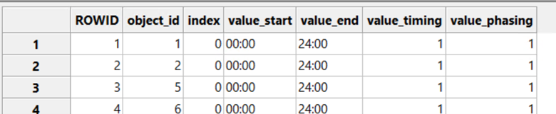
A node is signalized if it has active records in the table Signal. The Signal Nested Records determine the schedule (with start, end), timing and phasing that will be prevailing during a POLARIS Simulation. Some records are shown in the table below. Observe that one could have set a value_end prior to 24:00; in that case, it would be possible to add a record with the start as the end of the previous plan with another timing and phasing.
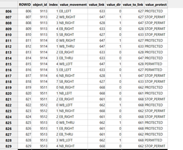
Now let’s focus on the timing and phasing definition. The Phase table resembles the table above connecting movements and phases. Note, however, a given intersection can take different phasing definition (for instance, having a permitted phase for left turns at certain times of the day only). As the screenshot below shows, the phasing definition connects movement and the phase id. In this table if a particular movement is not set, it is set as STOP. The value_movement (direction_turn_type) is usually automatically filled up by the QGIS plugin. The value_movement is used for determining conflicting movements. The Figure below has multiple records. Observe, for example, the row starts with 95 (9511, 9512, 9513). These are 3 phases associated with a phasing identifier. The link, direction and target link determines the associated connection to the movement.
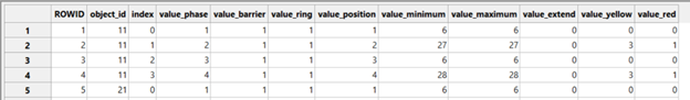
Finally, the actual timing definition, that is, for how long each phase will last. This is determined in the timing definition and sample is seen below for fixed time definition. The value_minimum is set equal to maximum and there is no extension along with yellow and red time. In the case of actuated signal control (currently unavailable), one could set maximum green time and the extension time.
Key parameters applicable to all supported models#
Aside the traffic model, these parameters are valid regardless:
simulation_interval_length_in_second: This integer value determines the traffic time step unless overridden by a particular traffic flow model.
num_simulation_intervals_per_assignment_interval: the product simulation_interval_length_in_second * num_simulation_intervals_per_assignment_interval determines the time-step in which the metrics are reported. For example, if the simulation_interval is 1 second and the num_simulation_interval is 60, the metrics will be reported every 60 seconds.
traffic_scale_factor (from 0 to 1): used for scaling the network properties in line with a sampling of the population synthesis. For instance, if traffic_scale_factor is 0.25 the effective capacity and jam density will be multiplied by this value. In other words, each vehicle “will count as four”.
use_traffic_api (false or true) / traffic_api_dll: this allows for user-defined code to be run along with POLARIS. Its specific behavior may depend on the underlying traffic flow model (mesoscopic, lagrangian,etc.).